Logistic regression boolean operators

Logistic regression을 이용하여 Boolean operators의 입력값에 따른 참/거짓 예측 모델 만들기

1. 개요

Logistic regression을 이용해 각 Boolean operators의 결과값을 예측하는 모델들을 제작한다. 모델들은 수업시간에 배웠던 예제를 활용하였다.

2. Source code

import random
import numpy as np
import seaborn as sns
import matplotlib.pylab as plt
plt.rcParams["figure.figsize"] = (5,5)

• numpy array를 가중치와 편향, x 변수에 이용하고 exp, log값을 계산하기위해 numpy 모듈을 임포트한다.
• 각 모델들의 cost 값을 그래프로 표현하기위해 seaborn 과 matplotlib 모듈을 임포트한다.

class logistic_regression_model():
    def __init__(self, Y):
        self.w = np.array([random.random(), random.random()])
        self.b = np.array(random.random())
        self.X = np.array([(0,0), (0,1), (1,0), (1,1)])
        self.Y = Y
        self.costArray = []

    def sigmoid(self, z):
        return 1/(1 + np.exp(-z))

    def predict(self, x):
        #z = self.w[0] * x[0] + self.w[1] * x[1] + self.b
        z = np.inner(self.w, x) + self.b
        a = self.sigmoid(z)
        return a

    def train(self, lr = 0.1):
        #dw0 = 0.0
        #dw1 = 0.0
        dw = np.array([0.0, 0.0])
        db = np.array(0.0)
        m = len(self.X)
        cost = 0.0

        for x, y in zip(self.X, self.Y):
            a = self.predict(x)
            if y == 1:
                cost -= np.log(a)
            else:
                cost -= np.log(1-a)

            #dw0 += (a-y)*x[0]
            #dw1 += (a-y)*x[1]
            dw += (a-y)*x
            db += (a-y)

        cost /= m
        #model.w[0] -= lr * dw0/m
        #model.w[1] -= lr * dw1/m
        self.w -= lr * dw/m
        self.b -= lr * db/m
        self.costArray.append(cost)

        return cost

각 모델을 구성하는 클래스 코드이다.

• math 모듈의 exp, log 함수를 numpy 의 exp, log 함수로 변경하였다.

def __init__(self, Y):
    self.w = np.array([random.random(), random.random()])
    self.b = np.array(random.random())
    self.X = np.array([(0,0), (0,1), (1,0), (1,1)])
    self.Y = Y
    self.costArray = []

• 클래스를 선언할 때 각 operator의 Y값(라벨)을 인자로 전달한다.
• 가중치와 편향을 난수로 구성된 numpy array로 변경하였다.
• x 변수를 numpy array로 변경하였다.
• 각 epoch에서 계산된 cost값을 저장하고 그래프로 표현하기위해 costArray를 생성하였다.

def predict(self, x):
    #z = self.w[0] * x[0] + self.w[1] * x[1] + self.b
    z = np.inner(self.w, x) + self.b
    a = self.sigmoid(z)
    return a

• 모델의 가중치와 x의 값의 수식 계산을 편리하게 하기위해 numpy inner product(내적)을 활용하였다.

def train(self, lr = 0.1):
    #dw0 = 0.0
    #dw1 = 0.0
    dw = np.array([0.0, 0.0])
    db = np.array(0.0)
    m = len(self.X)
    cost = 0.0

    for x, y in zip(self.X, self.Y):
        a = self.predict(x)
        if y == 1:
            cost -= np.log(a)
        else:
            cost -= np.log(1-a)

        #dw0 += (a-y)*x[0]
        #dw1 += (a-y)*x[1]
        dw += (a-y)*x
        db += (a-y)

    cost /= m
    #model.w[0] -= lr * dw0/m
    #model.w[1] -= lr * dw1/m
    self.w -= lr * dw/m
    self.b -= lr * db/m
    self.costArray.append(cost)

    return cost

• train 함수를 호출할 때 learning rate 값을 인자로 받는다. 기본값은 0.1이다.
• 각 가중치와 편향의 미분값을 계산할 변수들(dw0, dw1, db)을 numpy array로 변경하였다.
• numpy array를 활용하였기 때문에 가중치의 미분을 계산하는 두 줄의 코드를 한 줄의 코드 dw += (a-y)*x 로 통합할 수 있다.
• 마찬가지로, 각 가중치를 업데이트하는 두 줄의 코드도 한 줄의 코드 self.w -= lr * dw/m 으로 통합할 수 있다.

AND_model = logistic_regression_model([0, 0, 0, 1])
OR_model = logistic_regression_model([0, 1, 1, 1])
XOR_model = logistic_regression_model([0, 1, 1, 0])

for epoch in range(10000):
    AND_model.train(3)
    OR_model.train(3)
    XOR_model.train(3)

• 각 Boolean operator의 모델 클래스를 만들고 Y값(라벨)을 인자로 전달한다.
• epoch를 1만회로 설정하고 반복하여 모델을 학습한다.
• 각 모델의 train 함수를 호출하고 learning rate 3을 인자로 전달한다.

3. Cost plot

fig, line = plt.subplots(1, 3, figsize=(15,5))
fig.suptitle("Models cost plot at lr=3")

sns.lineplot(ax=line[0], data=AND_model.costArray)
line[0].set_title("AND model cost plot")
line[0].set_ylim(bottom=0, top=1)

sns.lineplot(ax=line[1], data=OR_model.costArray)
line[1].set_title("OR model cost plot")
line[1].set_ylim(bottom=0, top=1)

sns.lineplot(ax=line[2], data=XOR_model.costArray)
line[2].set_title("XOR model cost plot")
line[2].set_ylim(bottom=0, top=1)

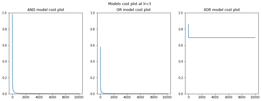
• AND model의 경우, cost값이 약 1.0으로 시작하여 epoch가 증가할수록 0에 가까워진다.
• 마찬가지로 OR model의 경우, cost값이 약 0.6으로 시작하여 epoch가 증가할수록 0에 가까워진다.
• 하지만 XOR model의 경우, cost값이 약 0.9로 시작하여 epoch가 증가하여도 약 0.5에서 증감되지않는 모습을 보인다.

4. Predicted result

print("   X\t      AND_model\t               OR_model\t      XOR_model")
for i in [(0,0), (0,1), (1,0), (1,1)]:
    print(f"{i} : {AND_model.predict(i)},\t {OR_model.predict(i)},\t {XOR_model.predict(i)}")

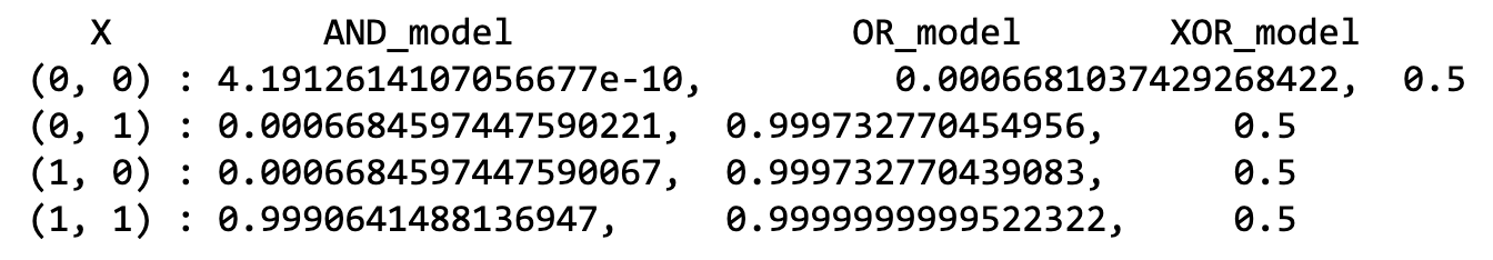
위의 결과를 확인해보면 AND 모델과 OR 모델은 잘 학습되어 올바른 예측 결과를 도출하였다. 하지만 XOR 모델에서는 모든 예측 결과가 0.5로 조금 이상한 모습을 보인다.